MaxHydro Input/Output

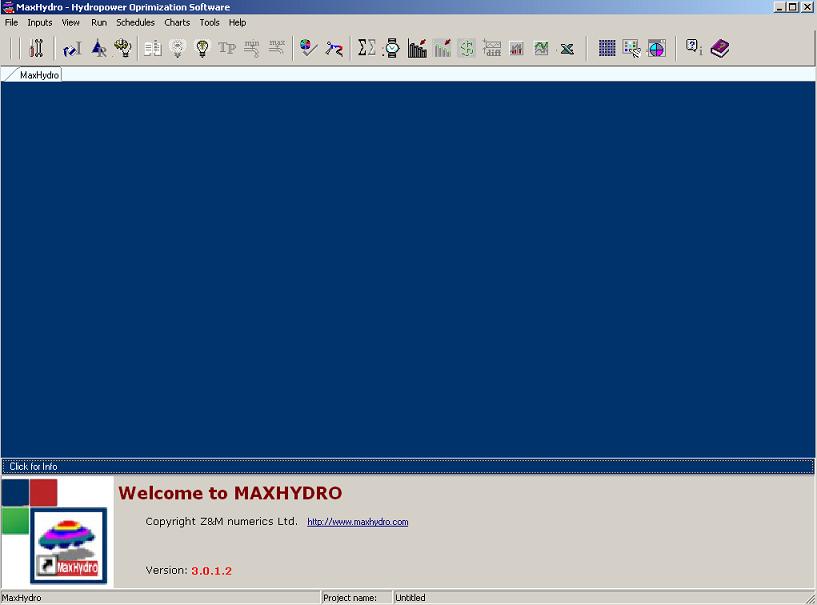
Optimization Process Flow

Step 1		Define the Optimization Problem and Select Options and Constraints.
Step 2		Define the System, Reservoir, Power Station data.
Step 3		Input Inflows, Tariffs and other time series data.
Step 4		Input efficiency for each generating unit as a function of head and discharge.
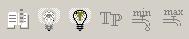
Step 5		Use these icons to generate and view the station efficiency matrix.
Step 6		Click to Run MaxHydro optimization module and to solve the optimization problem. The results from the run are written in a series of text files in the MaxHydro folder.
Step 7		Summury of the optimization results, total and average power produced, total and average inflows used, total and average release through the system, total and average benefits and other important results.
Scheduled view of all important results for each time step		Summary results for each time step presented in a schedule dialog. The end user can navigate forward or backwards and the summary data is presented in the dialog.
Output results, graphical post processor		There are numerous charts to show the optimal results. Charts for inflows and optimal discharges, power, efficiency differences, spilled water, benefits and tariffs, and other useful charts to show the optimal results. In addition all optimal data can be opened in excel for customized post processing.

Input data and parameters

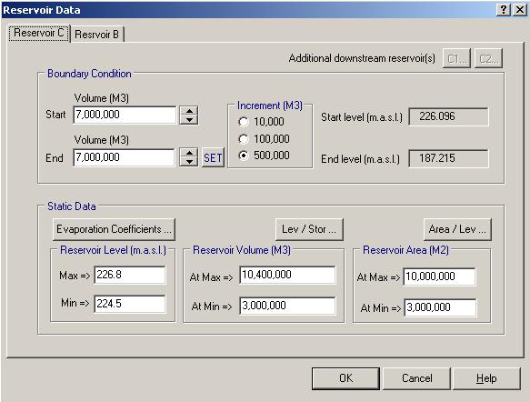
Reservoir data, maximum reservoir level and minimum reservoir level, the storage between the levels and the area of the reservoir.

 

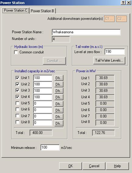
Power station data, including power station name, number of units and installed capacity.

Hydraulic Losses

The power conduit in some power stations can be common for all or some generating unit if this is the case then select the common conduit option and define the hydraulic loss function for a single conduit. Otherwise use the loss functions for each individual conduit (if common conduit is not selected)

Common Conduit

Select this option if common conduit is used for all the generating units, and define the hydraulic loss as a function of discharge: dh=f(Q), where dh is the hydraulic losses in (m) and Q is the station discharge in (cms).

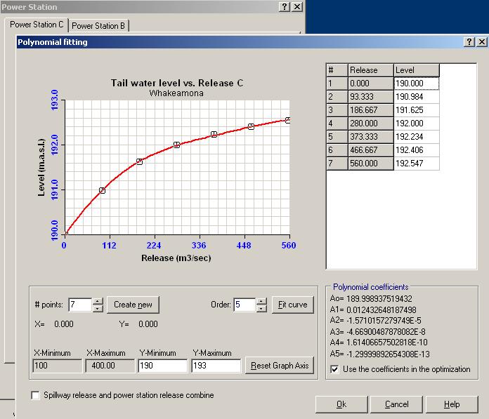
Tail Water Level To define the hydraulic loss function follow these steps:

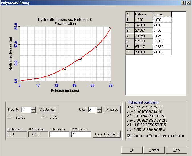
1. X-axis minimum and maximum values are defined based on the installed capacity (entered on the Power Station definition) for the individual unit or all units (if is common conduit).

2. Define the Y-axis as the minimum and maximum values for the hydraulic losses. Check and input correct values for the axis of the graph area where the loss function will be drawn. Click on the "Reset Graph Axis" button, to set the values for each axis on the drawing area above.

3. Select the number of points to represent the function dh=f(Q) and click the "Create new" button. In the example above, 7 points will be created. Any number greater than or equal to 5 can be used.

4. Click and drag each point vertically on the drawing area to the desired value. The grid on the right hand side of the graph holds the values for the points drawn on the graphical area. Alternatively input the values directly on the grid to the right. Only values for dh can be entered, the values for the discharge are fixed and cannot be changed. If you need more values for Q then use more points to represent the function.

5. Select now the polynomial function to fit through the points on the drawing area by choosing the order number (usually values from 3 to 5). Click the "Fit curve" button. This operation will fit polynomial function through the points on the drawing area and all coefficients will be displayed on the right bottom corner.

6. Make sure to tick the box "use the coefficients in the optimization". This will save the coefficients to a text file which then be used by the optimization module.

Separate conduits

If the power station has separate conduits define the hydraulic loss function to each generating unit. Select how many generating units are available for the optimization, tick the check box next to each available unit. Enter the maximum capacity of the unit in (cms) The approximate value of the power in (MW) is calculated based on the values of the maximum reservoir level, the value for the tail water level and using the efficiency value specified in the edit box "Average efficiency" at the bottom of the dialog. These values are approximate only and are not used in the optimization process.

Click on the "Dh..." button next to each unit to add the values for the hydraulic losses using the same procedure as described above for common conduit.

The next required step is to define the tail water level function.

1. Enter the TWL, tail water level at zero flow in (m), this is the level of the bottom of the tail water level structure. To define this function click the "Tail Water Levels..." button.

2. Follow the same process as described above to draw the graph and fit the polynomial curve.

3. Make sure to tick the box "use the coefficients in the optimization". This will save the coefficients to a text file which then be used by the optimization module.